This document describes how dense geospatial raster data can be represented using the W3C RDF Data Cube (QB) ontology [[vocab-data-cube]] in concert with other popular ontologies including the W3C/OGC Semantic Sensor Network ontology (SSN) [[vocab-ssn]], the W3C/OGC Time ontology (Time) [[owl-time]], the W3C Simple Knowledge Organisation System (SKOS) [[skos-reference]], W3C PROV-O [[prov-o]] and the W3C/OGC QB4ST [[qb4st]]. It offers general methods supported by worked examples that focus on Earth observation imagery.
Current triple stores, as the default database architecture for RDF, are not suitable for storing voluminous data like gridded coverages derived from Landsat satellite sensors. However we show here how SPARQL queries can be served through an OGC Discrete Global Grid System for observational data, coupled with a triple store for observational metadata.
While the approach may also be suitable for other forms of coverage, we leave the application to such data as an exercise for the reader.
For OGC This is a Public Draft of a document prepared
by the Spatial Data on the Web Working Group (SDWWG)
— a joint W3C-OGC project (see charter).
The document is prepared following W3C conventions. The document is
released at this time to solicit public comment.
Introduction
Publishing data on the Web using Linked Data
technologies makes it more accessible, easier to discover, and machine-readable. In the context of the rapidly growing availability and importance of earth observation data, this work aims to leverage the Linked Data approach to data publishing to make such data both much more easily usable by non-specialists and much more easily integrated with other Web data in applications.
Linked Data has worked well for multi-dimensional statistical data using the RDF Data Cube [[vocab-data-cube]]. Following this success, Earth Observation imagery can be readily modelled as a Data Cube with the three dimensions of latitude, longitude, and time. This simple conceptualisation and its encoding as Linked Data may be convenient for scientists and consumer app developers everywhere, and especially to statisticians such as those in National Statistics Organisations.
Satellite imagery is commonly modelled as a multidimensional grid coverage, as discussed in [[sdw-bp]].
The large number of data points that is typical of coverage data such as Landsat imagery means that publishers may be justifiably reluctant to address the size explosion that accompanies converting data to RDF. While such a conversion provides maximum machine-readability, many benefits of Linked Data can be realized with a compromise approach where only the metadata is directly expressed in RDF. Further benefits can be realized by storing voluminous gridded coverage data in more efficient storage representations and using specialised middleware to generate an RDF representation on-the-fly to respond to service requests.
This document illustrates that approach showing how Earth Observation imagery can be published as Linked Data using the RDF Data Cube vocabulary [[vocab-data-cube]] in concert with other relevant ontologies including the W3C/OGC Semantic Sensor Network ontology (SSN) [[vocab-ssn]], the W3C/OGC Time ontology (Time) [[owl-time]], the W3C Simple Knowledge Organisation System (SKOS) [[skos-reference]], W3C PROV-O [[prov-o]] and the W3C/OGC QB4ST [[qb4st]]. We show how SPARQL queries can be served through a scalable OGC Discrete Global Grid System for observation data, coupled with a triple store for observational metadata.
Throughout the document we refer to relevant Use Cases and Requirements of the Spatial Data on the Web Working Group (UCR) [[sdw-ucr]] and Best Practices of the Spatial Data on the Web Working Group (BP) [[sdw-bp]]. Those references may be helpful to provide real-world applications and further rationale for the approach described here. We refer to extracts from a small example for illustration. The complete source file for the example is
ANU-LED example.
The RDF Data Cube
The RDF Data Cube [[vocab-data-cube]] is a standard for representing multidimensional data as RDF.
It is typically used for numerical data that is associated with geographic regions (e.g. suburbs) and classifications (e.g. age, industry, or time periods).
Common practice includes using the SKOS vocabulary to define the concepts being reported
[Observed property in coverage].
The RDF Data Cube vocabulary allows the publisher to define all the relevant components of their data and the concepts they quantify,
including:
:lat a qb:DimensionProperty ;
    rdfs:subPropertyOf geo:lat .

:long a qb:DimensionProperty ;
    rdfs:subPropertyOf geo:long .

:time a qb:DimensionProperty ;
    rdfs:range xsd:dateTime ;
    qb:concept sdmx-concept:timePeriod .

:dataPixelValue a qb:MeasureProperty ;
    rdfs:range xsd:integer ;
    qb:concept :reflectance ;
    qb:concept sdmx-concept:obsValue .

# in pixels per degree
:resolution a qb:AttributeProperty ;
    rdfs:range xsd:double .
The ontology QB4ST [[qb4st]] extends the Data Cube for extra power and consistency when describing spatio-temporal aspects of data. [Georeferenced spatial data].
Any number of such dimensions can be defined, allowing for 1D, 2D, 3D or 4D coverages [Support for 3D, Time series, 4D model of space-time].
Traditionally, there is a distinction between data, that is the observations proper such as Landsat pixels and metadata,
which adds context to the observations such as resolution. In Linked Data modelling, this distinction is not strict.
However, it is possible to separate the two in a typical Data Cube.
The value of an RDF Data Cube component can be attached to each individual observation or to the dataset as a whole.
Dataset-wide metadata can therefore be distinguished from the rest of the dataset, because it is attached to the qb:DataSet object.
This makes it easy to fetch the metadata alone with a simple SPARQL query. This dataset-wide description alone is already a useful
(and web-of-data friendly) approach to publishing spatial data
[Spatial metadata].
The RDF Data Cube also enables much more detailed metadata, like
separate provenance for each observation. While it is not practical
to serve Landsat imagery with such detailed metadata attached to each
pixel, it may be reasonable to attach such metadata to
aggregated tiles of pixels. In this case, each
qb:Observation will be a whole tile
(:GridSquare) rather than an individual pixel [Support for
tiling]. Note that this technique applies BP Use
globally unique persistent HTTP URIs for spatial things at the
level of image tiles.
In the ideal web of data, every single observation has a unique URI, can be queried using SPARQL, and has metadata attached to it.
Upon hearing this, anyone familiar with Landsat data would be forgiven for rejecting the whole enterprise as entirely impractical.
But all is not lost! Most of the benefits of Linked Data (namely, linkability, enhanced discoverability, machine-readability) can
be realized by just publishing the dataset-wide metadata in this format. More 'linkiness' provides diminishing returns along with increasing costs.
Publishers must decide on the appropriate compromise position for their data.
To characterize the spectrum, we can broadly define three applications of RDF for coverages.
From most to least costly, these are: to store a coverage dataset, to serve a coverage (“serialization”), and to describe the metadata of a coverage (“description”).
Storing a coverage
RDF data is typically stored natively in a triple store. The Data Cube, and RDF in general, are too verbose to be viable for storing large coverages.
Serving a coverage
In this model, coverage data is physically stored in some more appropriate
format (such as HDF5). Specialized middleware implements a virtual triple store by receiving SPARQL
queries from a client and responding with
dynamically-generated RDF. Such a response may be verbose, but
the cost is much lower than physically storing the whole coverage
as RDF. Query optimization is also necessary for this to be
viable. Furthermore, we suggest using tiles for each
qb:Observation in the RDF Data Cube, rather than
individual pixels [Support for
tiling]. This significantly reduces the blowup that comes from
encoding data as RDF [Compressible].
The key advantage of serving a coverage in RDF is that the entire
coverage, and individual tiles within it, become linkable [Linkability];
this could be a major contribution to the Linked Data Web. With
sufficiently advanced middleware, SPARQL queries over the dataset
can be served just as if the data were stored in RDF, but for a
fraction of the storage cost. Not only that, but it is
possible to make direct SPARQL queries performant through use of
spatial data structures and assumptions about data layout, as
explained in Implementation. Hence,
it is still possible for publishers of dense spatial data to
leverage much of the power of linked data.
It is common to want only a chunk of the data available, for
example, all observations within 10km of Canberra in the past
year, as required for BP [ Expose spatial data through 'convenience APIs']. Regardless of the format chosen, an ability to assign
persistent identifiers to these sorts of queries is essential to
publishers of coverages. Although the RDF Data Cube offers
predefined chunks of triples called qb:slices for this
purpose, coverage applications typically demand a greater degree
of flexibility. Our approach is to let the publisher define
appropriate chunks [Reference
data chunks] using SPARQL queries. For example,
FILTERs with inequalities can be used to return all
tiles of a particular resolution within a particular spatial rectangle.
If using this method to denote chunks, publishers should make
it easy for a user to select chunks without the use of SPARQL directly,
e.g. by providing an interface to generate the appropriate query
using a few predefined operators.
Whatever approach is taken, it should be as easy as possible
for the user to grab just the metadata, without having to figure out how to write an appropriate query.
The definition of a qb:DataSet and the associated qb:DataStructureDefinition can serve this role, but it is still up to the
publisher to make it easy for the user to download those definitions.
It is also helpful if the user can easily identify the domain of a coverage, that is, the spatial and temporal area where measurements are made
[Spatial metadata].
QB4ST [[qb4st]] does not currently have a term for that, but it might in the future.
Discrete global grid systems are a family of spatial reference systems that subdivide the Earth's surface into a hierarchy of cells.
Larger cells are subdivided into smaller cells deeper in the hierarchy.
A location on the Earth's surface is specified by a cell id, not a latitude and longitude. Smaller cells are more precise, so choosing a cell forces the publisher to include a measure of uncertainty for any spatial measure.
Cells are convenient units of tiling for gridded coverages. Each pixel in a tile corresponding to a larger cell can represent a measurement made on a smaller cell in the hierarchy below.
The OGC published a standard specification of DGGS in August 2017 as ”Topic 21: Discrete Global Grid Systems Abstract Specification” [[OGC-15-104r5]].
The ANU-LED example in this document does not require the use of a DGGS. However, the DGGS has some convenient properties that make it particularly suitable for Linked Data.
First, each DGGS cell
has a unique identifier, so it is easy to generate natural URIs for each chunk of data.
Second, the DGGS we use, rHEALPix [[rHealPIX]],
defines cell geometries so that cells at the same level of the
hierarchy have equal areas. This makes rHEALPix a suitable format for
storing multiple datasets at different resolutions, or several different
resolution views of the same dataset. The equal-area constraint means that
different resolution pixels are directly comparable, and no resampling is
required [Avoid
coordinate transformations], as advised by BP Choose the coordinate reference system to suit your user's applications. Third, the hierarchical nature of the
DGGS makes it convenient to implement spatial optimizations when responding
to queries, by pruning the tree early to eliminate whole regions of
unpromising cells that fall outside the desired area.
Data structures other than DGGS are also amenable to these approaches, for example n-dimensional gridded data, whether geospatial or not, and hierarchical structures such as tile sets, octrees and quadtrees.
Scalable Implementation
A proof of concept demonstrating the ANU-LED example with a SPARQL query
system employing rHEALPix to retrieve satellite imagery has been implemented. This
section briefly describes some of the strategies employed to make
the implementation efficient. All code referenced here is available
on GitHub [[led-github]].
As discussed previously, scalable implementations of a Data Cube
for Earth observations must grapple with the verbosity of RDF
representations relative to specialized coverage formats like GeoTIFF. This
precludes materializing the entire dataset as RDF, storing it on
disk, and serving it using an off-the-shelf triple store. Instead,
implementations must employ a “virtual graph”, which can
be used to service SPARQL queries without materializing all triples
in advance. This approach has precedent: virtual graphs have been used
to provide linked data interfaces to relational databases, RSS
feeds, and ordinary HTML pages with no semantic markup
[[perf-vgraph]].
For the purpose of illustrating how triple stores service SPARQL
queries—regardless of whether they are backed by virtual or
materialized graphs—consider the query below.
SELECT ?s ?v WHERE {
    ?s a :egType ;
        rdfs:label "Example" ;
        :value ?v .
    FILTER (?v < 15)
}
The heart of the query above is a Basic Graph Pattern (BGP) which
specifies the triples to be accessed. In this case,
the BGP contains three patterns. Written explicitly, they are:
Conceptually, a triple store will service the query above by
iterating through each triple pattern in turn. First, a set of
bindings for ?s will be generated that are consistent
with ?s a :egType. That set of bindings will then be
filtered by matching them against the pattern ?s rdfs:label
"Example". The final ?s :value ?v will further
filter the bindings for ?s by considering only subjects
?s with a :value property; it will also
introduce a corresponding set of bindings for ?v.
Having generated all bindings relevant to the BGP, a typical triple
store will then apply the FILTER condition to each. This
general approach works for both traditional storage backends (like
on-disk RDF databases) and non-traditional ones (like virtual
graphs).
In practice, processing each element of a SPARQL query sequentially
is too inefficient to be of use in a large database. Instead, triple
stores employ a range of optimisations to combine steps of
the query process, speed up selected operations, or minimise the
number of bindings produced by each stage, as outlined in
[[sparql-opt]]. For example, a triple store could speed up matching
triples of the form ?s a :egType by keeping an index of
all URIs associated with each present rdf:type, or
could accelerate BGP matching by reordering the pattern to ensure
that the most restrictive patterns are evaluated first.
Although we do not materialise our RDF triples, similar techniques
are applicable to our virtual graph middleware. As a simple
illustration of the optimisation opportunities available, we have
implemented two simple optimisations:
User-supplied triple patterns often generate highly selective constraints
on the data returned by a SPARQL query. For example, the pattern
?s :dggsLevelSquare 5 . allows a virtual graph
implementation to ignore all observations not corresponding to cells
at the fifth level of the DGGS hierarchy. In a naive
implementation, only one such BGP can be considered at a
time; this makes strategies for BGP ordering essential. In
contrast, a virtual graph query processor can simultaneously
consider all supplied constraints in conjunction. For
instance, if the user specifies ?s :dggsLevelSquare 5;
:etmBand 3, then the virtual graph implementation can
safely narrow its search to observations at level 5 of the DGGS
hierarchy which correspond to Landsat's third ETM band.
Consumers of spatial datasets typically request only a small
spatial rectangle of the available data. In SPARQL, such a rectangle can
be identified by a FILTER statement restricting the
appropriate location properties. By inspecting the contents of
FILTER statements, virtual graph implementations
can preemptively narrow the set of bindings they generate to
include only bindings which are spatially relevant. In general,
this approach can yield excellent gains when the spatial extent
of queries is small relative to the spatial extent of the
overall dataset, which is typical of Earth Observation imagery.
These simple optimizations can improve query time substantially.
Consider the following SPARQL query, which fetches the intensity
(?val) and URI (?s) associated with each
single-pixel observation in a satellite imagery database. Note the
use of custom :latMin and :longMax to
define the edges of a bounding box—we have included these in
our demonstration system for ease of implementation, but it is
expected that in a production system would use GeoSPARQL-style
FILTERs together with the WKT-formatted
:bounds predicate used elsewhere in this document.
SELECT DISTINCT ?s ?val WHERE {
    ?s a :Pixel
        :etmBand "1"^^xsd:int ;
        :dggsLevelSquare "5"^^xsd:int ;
        # See comment above on :latMin/:longMax
        :latMin ?latMin ;
        :longMax ?longMax ;
        :dataPixelValue ?val .
    # Everything north-west of Parliament House
    FILTER (?latMin > -35.3082
        && ?longMax < 149.1244)
}
The above query was executed on a 500MB HDF5 dataset containing over
4000 distinct observations. Repeating the query a thousand times
with ten concurrent clients on a desktop machine yielded the
following mean running times. In the following, the “naive” implementation
simply iterates through the BGP specified above on a
pattern-by-pattern basis, subsequently passing results to
the SPARQL engine for evaluation against the filter constraint.
“Multiple pattern-matching” corresponds to the first
optimization identified above, and “additional spatial
optimizations” refers to a combination of the first and second
optimizations.
Implementation
Mean runtime (± standard deviation)
Naive
378ms (±65.5ms)
…with multiple-pattern matching
35ms (±22.2ms)
…with additional spatial optimisations
17ms (±11.8ms)
“Multiple-pattern matching” is a relatively simple
optimization, yet is sufficient to improve query performance
tenfold. Accounting for the bounding box constraint specified in the
query improves performance by another factor of two. It is likely
that further performance gains could be found with more
sophisticated optimizations. In particular, processing queries with
general polygonal spatial constraints could be further improved by employing an
R-tree or some other specialized spatial data structure.
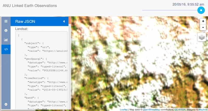
To demonstrate the practical utility of our system, we produced a
simple web-based client application. The client application is able
to fetch Landsat imagery and its associated metadata via SPARQL
queries. It can then overlay the retrieved images on a movable map.
As mentioned previously, code for both the client and sever is
available on GitHub [[led-github]].
A screenshot of the client application running in a browser.
Use of existing ontologies
RDF makes it easy to re-use terms defined in external ontologies and some of the most widely applicable are explained here. See the
ANU-LED example for some specific examples of these.
SSN
The Semantic Sensor Network ontology [[vocab-ssn]] defines terms which can be used to describe satellite sensors that collect Earth observation data
[Sensor metadata].
The ANU-LED example
illustrates a minimal description of Landsat 8 OLI observations using SSN
[SSN-like representation].
Much more detailed descriptions are possible. In particular, SSN descriptions can be attached to individual tiles
[Quality per sample], demonstrating BP Include spatial metadata in dataset metadata.
The PROV ontology [[prov-o]] allows the provenance of data to be traced
[Provenance].
It provides terms for describing what entities the data is based on,
what processes were used to convert those entities into others and into the final data,
and what individuals and organisations were responsible for those processes.
PROV-O descriptions can be attached at the dataset level, and also at the individual
observation or tile level to indicate precisely from which source material each observation is derived.
Spatial data best practice eschews unqualified uses of “latitude” and “longitude”.
Commonly, these terms refer to the WGS-84 Coordinate Reference System (CRS),
but data published according to BP State how coordinate values are encoded should always make its CRS explicit [Georectification].
In RDF, the WGS-84 geo vocabulary is often used,
with its provided geo:lat and geo:long properties.
QB4ST defines the qb4st:crs property to identify a CRS definition
[CRS definition, Spatial metadata].
The RDF Data Cube and QB4ST make is easy to define several CRSs and to use them simultaneously, providing clients with several views of the data [Multiple CRSs]. In the example below, a grid square can be identified by the latitude and longitude of its centroid, by its boundary, or by its rHEALPix cell.
The RDF Data Cube is commonly used in conjunction with a SKOS [[skos-reference]] concept scheme
(such as SDMX-RDF and its concept scheme)
to define the meanings of the components [Observed property in coverage].
It is appropriate to use this for coverages also, but appropriate SKOS concepts do not always exist.
They may need to be published along with the data proper.
Coverages should be annotated appropriately with the times observations were taken
[Coverage temporal extent], that is BP Describe properties that change over time.
OWL-Time [[owl-time]] defines terms for time intervals that are useful for expressing the temporal domain of the dataset.
It also allows temporal reference systems other than the Gregorian calendar.
However, for Gregorian time instants which are typically used for Earth observation data, a datatype property using the built-in xsd:dateTime datatype is sufficient.
QB4ST defines terms that work well together with OWL-Time.
This work would not be possible without the TechLauncher program of the Australian National University and its ardent convenor, Shayne Flint.
We also thank Matthew Purss of Geoscience Australia for participating in the program and supporting this project.
Finally, Ed Parsons of Google, Robert Woodcock of CSIRO, Robert Atkinson of the OGC and Bill Roberts of SWIRRL provided valuable discussions and feedback. The editors gratefully acknowledge the contributions of all members of the Spatial Data on the Web Working Group, its chairs Kerry Taylor and Ed Parsons, and W3C and OGC staff Phil Archer, Francois Daoust and Scott Simmons.